Let’s stick with the Volt meter example from yesterday, but use a parabolic model:
𝑦 = 𝑎 + 𝑑𝑥 (𝑏 + 𝑑𝑥 𝑐) 𝑑𝑥 = 𝑥 − 𝑥₀
The parameters 𝑎, 𝑏 and 𝑐 need to be determined during the calibration procedure.
| measurement number | 1 | 2 | 3 | 4 | 5 | 6 |
|---|---|---|---|---|---|---|
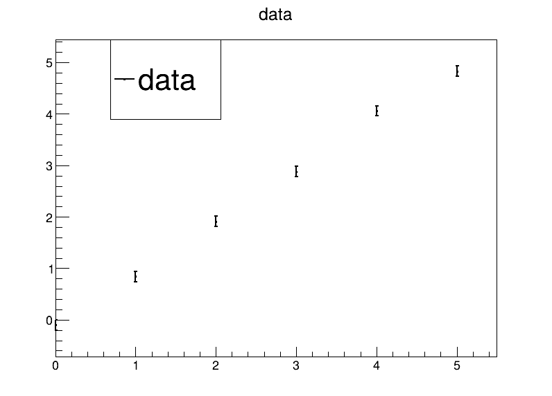
| reference 𝑥 (true) [V] | 0 | 1 | 2 | 3 | 4 | 5 |
| measured 𝑦 [V] | -0.10 | 0.84 | 1.91 | 2.88 | 4.06 | 4.83 |
The uncertainty for all measured voltages is 0.1 V.
Code up a visualisation of the data.
import ROOT

Vtrue = [0, 1, 2, 3, 4, 5]
V = [-.10, .84, 1.91, 2.88, 4.06, 4.83]
sigmas = [.1, .1, .1, .1, .1, .1]

ROOT.gROOT.SetBatch()
c = ROOT.TCanvas("c", "c", 800, 600)

# build graph with data
gdata = ROOT.TGraphErrors(len(Vtrue))
gdata.SetNameTitle("gdata", "data")
for i in range(0, len(Vtrue)):
    gdata.SetPoint(i, Vtrue[i], V[i])
    gdata.SetPointError(i, 0., sigmas[i])
gdata.SetLineWidth(2)
gdata.SetMarkerStyle(7)
gdata.SetMarkerSize(2)

gdata.Draw("AP")  # draw data

c.SaveAs("day2-ex1.pdf")
Given the model from the last slide,
𝑦 = 𝑎 + 𝑑𝑥 (𝑏 + 𝑑𝑥 𝑐) 𝑑𝑥 = 𝑥 − 𝑥₀
the χ² function comes out as
χ² = ∑ ᵢ (𝑦ᵢ − 𝑎 - 𝑑𝑥ᵢ 𝑏 - 𝑑𝑥ᵢ² 𝑐)²/2σᵢ²
We need to minimize that function with respect to the fit parameters 𝑎, 𝑏 and 𝑐.
χ² = ∑ ᵢ (𝑦ᵢ − 𝑎 - 𝑑𝑥ᵢ 𝑏 - 𝑑𝑥ᵢ² 𝑐)²/2σᵢ²
Calculate the derivative with respect to 𝑎, 𝑏 and 𝑐, and put them to zero.
χ² = ∑ ᵢ (𝑦ᵢ − 𝑎 - 𝑑𝑥ᵢ 𝑏 - 𝑑𝑥ᵢ² 𝑐)²/2σᵢ²
Putting the derivatives to zero yields:
0 = 𝜕χ²/𝜕𝑎 = ∑ ᵢ (𝑦ᵢ − 𝑎 - 𝑑𝑥ᵢ 𝑏 - 𝑑𝑥ᵢ² 𝑐)(  -1 ) / σᵢ²
0 = 𝜕χ²/𝜕𝑏 = ∑ ᵢ (𝑦ᵢ − 𝑎 - 𝑑𝑥ᵢ 𝑏 - 𝑑𝑥ᵢ² 𝑐)(-𝑑𝑥ᵢ ) / σᵢ²
0 = 𝜕χ²/𝜕𝑐 = ∑ ᵢ (𝑦ᵢ − 𝑎 - 𝑑𝑥ᵢ 𝑏 - 𝑑𝑥ᵢ² 𝑐)(-𝑑𝑥ᵢ²) / σᵢ²
0 = 𝜕χ²/𝜕𝑎 = ∑ ᵢ (𝑦ᵢ − 𝑎 - 𝑑𝑥ᵢ 𝑏 - 𝑑𝑥ᵢ² 𝑐)(  -1 ) / σᵢ²
0 = 𝜕χ²/𝜕𝑏 = ∑ ᵢ (𝑦ᵢ − 𝑎 - 𝑑𝑥ᵢ 𝑏 - 𝑑𝑥ᵢ² 𝑐)(-𝑑𝑥ᵢ ) / σᵢ²
0 = 𝜕χ²/𝜕𝑐 = ∑ ᵢ (𝑦ᵢ − 𝑎 - 𝑑𝑥ᵢ 𝑏 - 𝑑𝑥ᵢ² 𝑐)(-𝑑𝑥ᵢ²) / σᵢ²
In terms of our “shorthand”,
𝑎   ⟨1⟩  + 𝑏  ⟨𝑑𝑥⟩  + c ⟨𝑑𝑥ᵢ²⟩ =   ⟨𝑦⟩
𝑎  ⟨𝑑𝑥⟩  + 𝑏 ⟨𝑑𝑥ᵢ²⟩ + c ⟨𝑑𝑥ᵢ³⟩ =  ⟨𝑦 𝑑𝑥⟩
𝑎 ⟨𝑑𝑥ᵢ²⟩ + 𝑏 ⟨𝑑𝑥ᵢ³⟩ + c ⟨𝑑𝑥ᵢ⁴⟩ = ⟨𝑦 𝑑𝑥ᵢ²⟩
𝑎   ⟨1⟩  + 𝑏  ⟨𝑑𝑥⟩  + c ⟨𝑑𝑥ᵢ²⟩ =   ⟨𝑦⟩
𝑎  ⟨𝑑𝑥⟩  + 𝑏 ⟨𝑑𝑥ᵢ²⟩ + c ⟨𝑑𝑥ᵢ³⟩ =  ⟨𝑦 𝑑𝑥⟩
𝑎 ⟨𝑑𝑥ᵢ²⟩ + 𝑏 ⟨𝑑𝑥ᵢ³⟩ + c ⟨𝑑𝑥ᵢ⁴⟩ = ⟨𝑦 𝑑𝑥ᵢ²⟩
Or, in matrix form (let’s call the matrix below M):
/   ⟨1⟩   ⟨𝑑𝑥⟩  ⟨𝑑𝑥ᵢ²⟩ \ / a \     /   ⟨𝑦⟩    \
|  ⟨𝑑𝑥⟩  ⟨𝑑𝑥ᵢ²⟩ ⟨𝑑𝑥ᵢ³⟩ | | b |  =  |  ⟨𝑦 𝑑𝑥⟩  |
\ ⟨𝑑𝑥ᵢ²⟩ ⟨𝑑𝑥ᵢ³⟩ ⟨𝑑𝑥ᵢ⁴⟩ / \ b /     \ ⟨𝑦 𝑑𝑥ᵢ²⟩ /
| measurement number | 1 | 2 | 3 | 4 | 5 | 6 |
|---|---|---|---|---|---|---|
| reference 𝑥 (true) [V] | 0 | 1 | 2 | 3 | 4 | 5 |
| measured 𝑦 [V] | -0.10 | 0.84 | 1.91 | 2.88 | 4.06 | 4.83 |
The uncertainty for all measured voltages is 0.1 V. Using the model
𝑦 = 𝑎 + 𝑑𝑥 (𝑏 + 𝑑𝑥 𝑐) 𝑑𝑥 = 𝑥 − 𝑥₀
leads to the matrix equation
/   ⟨1⟩   ⟨𝑑𝑥⟩  ⟨𝑑𝑥ᵢ²⟩ \ / a \     /   ⟨𝑦⟩    \
|  ⟨𝑑𝑥⟩  ⟨𝑑𝑥ᵢ²⟩ ⟨𝑑𝑥ᵢ³⟩ | | b |  =  |  ⟨𝑦 𝑑𝑥⟩  |
\ ⟨𝑑𝑥ᵢ²⟩ ⟨𝑑𝑥ᵢ³⟩ ⟨𝑑𝑥ᵢ⁴⟩ / \ b /     \ ⟨𝑦 𝑑𝑥ᵢ²⟩ /
Write a piece of code to calculate the matrix and right hand side from the data.
def buildLinSystemForParabolaFit(xs, ys, sigmays, x0):
    rhs = [0, 0, 0]
    mat = [0, 0, 0, 0, 0, 0]
    for x, y, sigma in zip(xs, ys, sigmays):
        w = 1 / (sigma * sigma)
        dx = x - x0
        dx2 = dx * dx;
        rhs[0] += w * y
        rhs[1] += w * y * dx
        rhs[2] += w * y * dx2
        mat[0] += w
        mat[1] += w * dx
        mat[2] += w * dx2
        mat[4] += w * dx * dx2
        mat[5] += w * dx2 * dx2
    mat[3] = mat[2]
    return rhs, mat
A word on the routine on the last page is in order: It uses packed matrix storage. The matrix is symmetric, so it’s attractive to only save half of it.
Consider a symmetric 100 x 100 matrix (100 fit parameters can happen in practice). That means updating around 78 kiB of matrix elements for every measurement with normal martix storage. With packed storage, it’s only about 40 kiB of storage. For large matrices and/or large data sets, this translates into a nice speed gain.
Technically, one saves only the diagonale and below, and find element 𝑀ᵢⱼ in an array at index 𝑖 ⋅ (𝑖 + 1) / 2 + 𝑗 for (𝑗 <= 𝑖):
𝑀₀₀, 𝑀₁₀, 𝑀₁₁, 𝑀₂₀, 𝑀₂₁, 𝑀₂₂ …
A linear system of equations, 𝑀 𝐱 = 𝐛, is usually solved by using some matrix decomposition method. The strategy is usually to
write 𝑀 = 𝐾 𝑅 where
𝐾 is a matrix that is easily invertible
𝑅 is usually a upper right matrix, i.e. can be solved by substitution
/ 𝑅₁₁ 𝑅₁₂ ⋯ 𝑅ₙₙ \
𝑀 = K ⋅ | 0 𝑅₂₂ 𝑅₂ₙ | | ⋮ ⋱ ⋱ ⋮ | \ 0 ⋯ 0 𝑅ₙₙ /
𝐾⁻¹ is thus the matrix that annihilates the lower left half of 𝑅 (as 𝐾⁻¹ 𝑀 = 𝑅).
There are a number of common matrix decomposition strategies:
These methods have different properties regarding their numerical stability (more on that later).
Given a symmetric positive matrix 𝑀 = 𝑀ᵀ > 0, Cholesky decomposition forms a lower triangular matrix 𝐿. Example:
/   4  12 -16 \   /  2 0 0 \   / 2 6 -8 \
|  12  37 -43 | = |  6 1 0 | ⋅ | 0 1  5 |
\ -16 -43  98 /   \ -8 5 3 /   \ 0 0  3 /
For a general 𝑛 × 𝑛 real matrix M, the elements of 𝐿 can be computed as follows:
       ____________________
𝐿ⱼⱼ = √ 𝑀ⱼⱼ − ∑ ₖ₌₁ʲ⁻¹ 𝐿ⱼₖ²

𝐿ᵢⱼ = 1 / 𝐿ⱼⱼ (𝑀ᵢⱼ − ∑ ₖ₌₁ʲ⁻¹ 𝐿ᵢₖ 𝐿ⱼₖ)   for 𝑖 > 𝑗
A matrix 𝑀 is (alomst) never exact: floating point numbers have a finite precision, and often there are measurement uncertainties.
The matrix M itself is usually given by the problem, and we can not do anything about it. But the choice of matrix 𝐾 in the decomposition 𝑀 = 𝐾 𝑅 can make matters worse or better.
Let’s look at the eigenvalues (EV) of K, ordered by absolute value:
|λₘᵢₙ| = |λ₁| <= |λ₂| <= … <= |λₙ| = |λₘₐₓ|
The overall scale of the EV does not matter, because an overall scaling does not change the relative numerical error in the calculation of 𝑅 = 𝐾⁻¹ 𝑀 and 𝐫’ = 𝐾⁻¹ 𝐫.
The “eigenvalue contrast” or condition number κ = |λₘₐₓ| / |λₘᵢₙ| is what drives numerical stability because it determines an upper bound for the “amplification” of the numerical error along the directions of the eigenvectors.
What are typical values of the condition number κ?
𝐿𝑈 decomposition: depends on matrix 𝑀, but 10⁴…10⁶ not uncommon (single precision float has only 7 decimal digits precision!)
𝑄𝑅 decomposition: 𝑄 has only eigenvalues ±1 – numerically stable
SVD: uses two rotation/mirror matrices like 𝑄𝑅 – numerically stable
Cholesky decomposition:
/ 1 0 ⋯ 0 \ / 𝐷₁ 0 ⋯ 0 \ / 1 𝐿₂₁ ⋯ 𝐿ₙₙ
| 𝐿₂₁ 1 ⋱ 0 | | 0 𝐷₂ ⋱ 0 | | 0 1 ⋯ 𝐿₂ₙ |
| ⋮ ⋱ 0 | | 0 ⋱ ⋱ 0 | | 0 ⋱ ⋱ ⋮ |
\ 𝐿ₙ₁ 𝐿ₙ₂ ⋯ 1 / \ 0 ⋯ 0 𝐷ₙ / \ 0 ⋯ 0 1 /
       ____________________
𝐿ⱼⱼ = √ 𝑀ⱼⱼ − ∑ ₖ₌₁ʲ⁻¹ 𝐿ⱼₖ²

𝐿ᵢⱼ = 1 / 𝐿ⱼⱼ (𝑀ᵢⱼ − ∑ ₖ₌₁ʲ⁻¹ 𝐿ᵢₖ 𝐿ⱼₖ)   for 𝑖 > 𝑗
Implement Cholesky decomposition in code, and write a routine that allows to solve 𝑀 𝐱 = 𝐫 with two substitution passes.
Test the routine. Write a piece of code that uses the solver from above to invert a symmetric positive-definite matrix, and test it.
bool choleskyDecomp(unsigned n, double* m)
{
    PackedMatrixAdapter<double> M(m); // make packed storage accessible, see file
    for (unsigned j = 0; n != j; ++j) {
        double diag = M[j][j];
        for (unsigned k = j; k--; )
            diag -= M[j][k] * M[j][k];
        if (diag <= 0) return false;
        M[j][j] = diag = std::sqrt(diag);
        diag = 1 / diag;
        for (unsigned i = j + 1; n != i; ++i) {
            double tmp = M[i][j];
            for (unsigned k = 0; j != k; ++k)
                tmp -= M[i][k] * M[j][k];
            M[i][j] = tmp * diag;
        }
    }
    return true;
}
void solve(unsigned n, const double* l, double* b)
{
    PackedMatrixAdapter<const double> L(l);
    // solve L y = b
    for (unsigned i = 0; n != i; ++i) {
        double tmp = b[i];
        for (unsigned j = 0; i != j; ++j)
            tmp -= L[i][j] * b[j];
        b[i] = tmp / L[i][i];
    }
    // solve L^T x = y, save in b
    for (unsigned i = n; i--; ) {
        double tmp = b[i];
        for (unsigned j = n; --j != i;)
            tmp -= L[i][j] * b[j];
        b[i] = tmp / L[i][i];
    }
}
void invert(unsigned n, double* l)
{
    std::vector<double> mat(l, l + n * (n + 1) / 2);
    PackedMatrixAdapter<double> Li(l);
    std::vector<double> tmp;
    tmp.reserve(n);
    for (unsigned i = 0; n != i; ++i) {
        tmp.assign(n, 0);
        tmp[i] = 1;
        solve(n, mat.data(), tmp.data());
        for (unsigned j = 0; j <= i; ++j)
            Li[i][j] = tmp[j];
    }
}
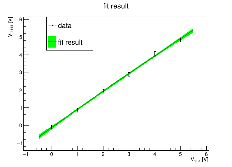
Take the code that calculates matrix and right hand side from earlier, and use the Cholesky code to solve the matrix equation, and work out the covariance.
If your Cholesky decomposition code does not work yet, look into numpy, ROOT, GSL or similar packages, and use their routines. (You have to know what these routines do, but in real life, you should likely use a library routine that’s well debugged…)
Visualize the results (like yesterday).
Ideally, one would like to assess how well one is doing with the fits. There are a couple of things we can look at:
Once the best fit point is known, we can calculate the χ² value for the data.
If things behave well, χ² should be about the number of degrees of freedom (ndf), i.e. the number of data points minus the number of fit parameters.
In other words, χ² / ndf should be around 1 for a good fit to more than a handful of data points.
Calculate χ² and χ² / ndf for your parabolic fit.
If the measurements are normally distributed, one can calculate from first principles how likely it is to get a certain value of χ² (given ndf).
The cumulative distribution function (CDF) measures how likely it is to get a χ² value that is at most as bad as the one observed. This is called the p-value.
          / χ²
p-value = |    𝑑χ'² 𝑃(χ'², 𝑛𝑑𝑓)
          / 0
In ROOT, you can access this function with ROOT.TMath.Prob(chi2, ndf).
What is the p-value for your fit?
def calcChi2(xs, ys, sigmas, x0, param):
    retVal = 0
    for x, y, s in zip(xs, ys, sigmas):
        w = 1 / (s * s)
        dx = x - x0
        ypred = param[0] + dx * (param[1] + dx * param[2])
        retVal += (y - ypred) * (y - ypred) * w
    return retVal

chi2 = calcChi2(xs, ys, sigmas, 2.5, crhs)
prob = ROOT.TMath.Prob(chi2, 3)

print("chi={} prob={}".format(chi2, prob))