The idea with toys or pseudo-experiments is to mimic the ability to run a fit on many simulated data sets.
For that, one can use a pseudo-random number generator or (P)RNG. It is “seeded” with a value (often the system time), and generates a long sequence of numbers (think order 10¹⁰⁰ numbers) that behave like uniformly distributed random numbers. Based on these, one can simulate various distributions.
In ROOT, you can use
rng = ROOT.TRandom3() # seed with system time
x = rng.Gauss(3., 2.) # generate random number, mean 3, sigma 2
to generate normally distributed random numbers.
Rewrite your parabolic fit to:
How do the plots look?
The code is a bit large-ish to include on slides, but it should be familiar by
now, and is available .
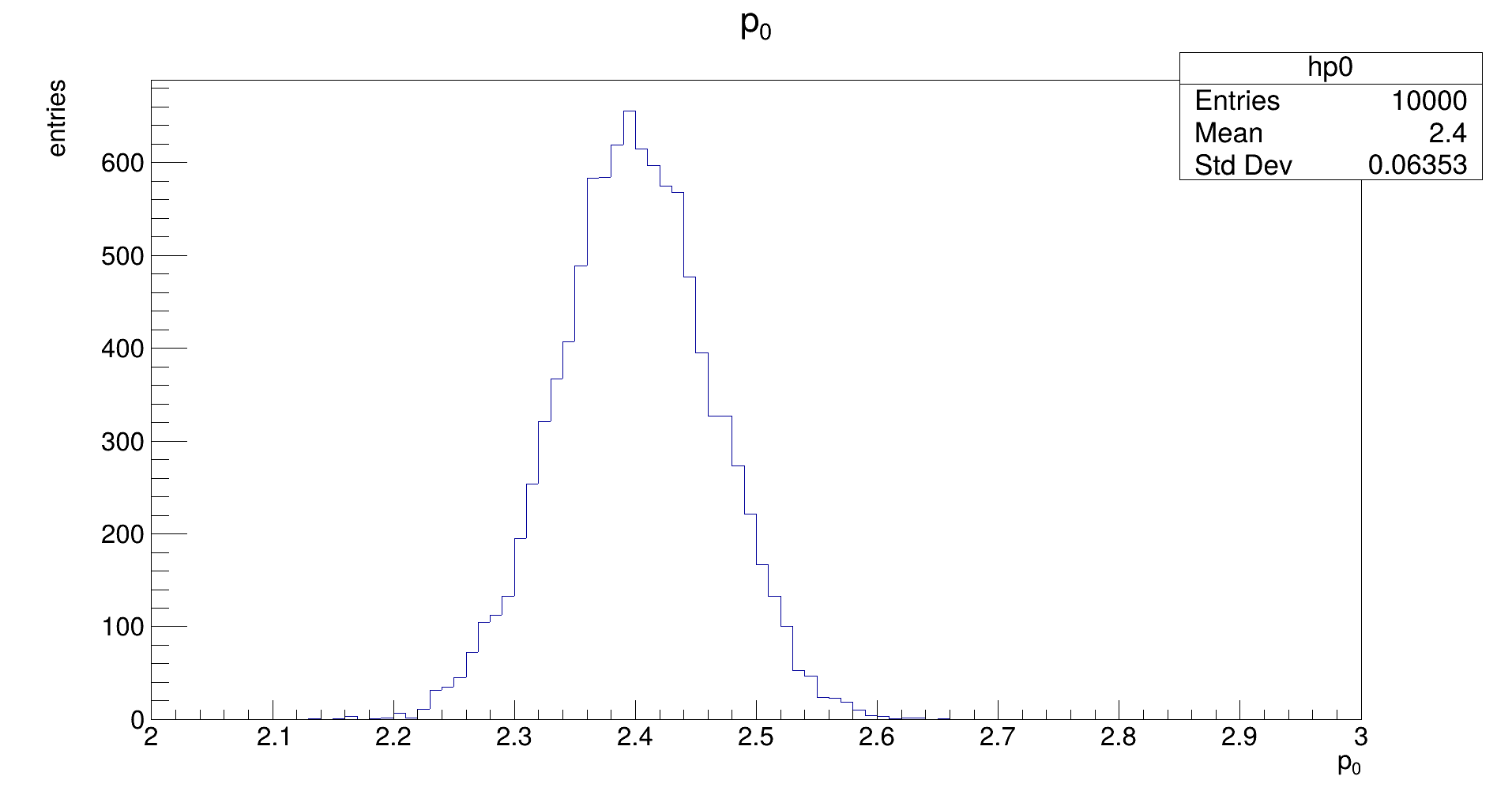
The distribution should be Gaussian, with a mean of the true (generation) value of 𝑝₀, and its width representing the uncertainty that is achievable with the fit. (Note: the latter does not need to be the same as the uncertainty that is estimated by the fit in the covariance.)
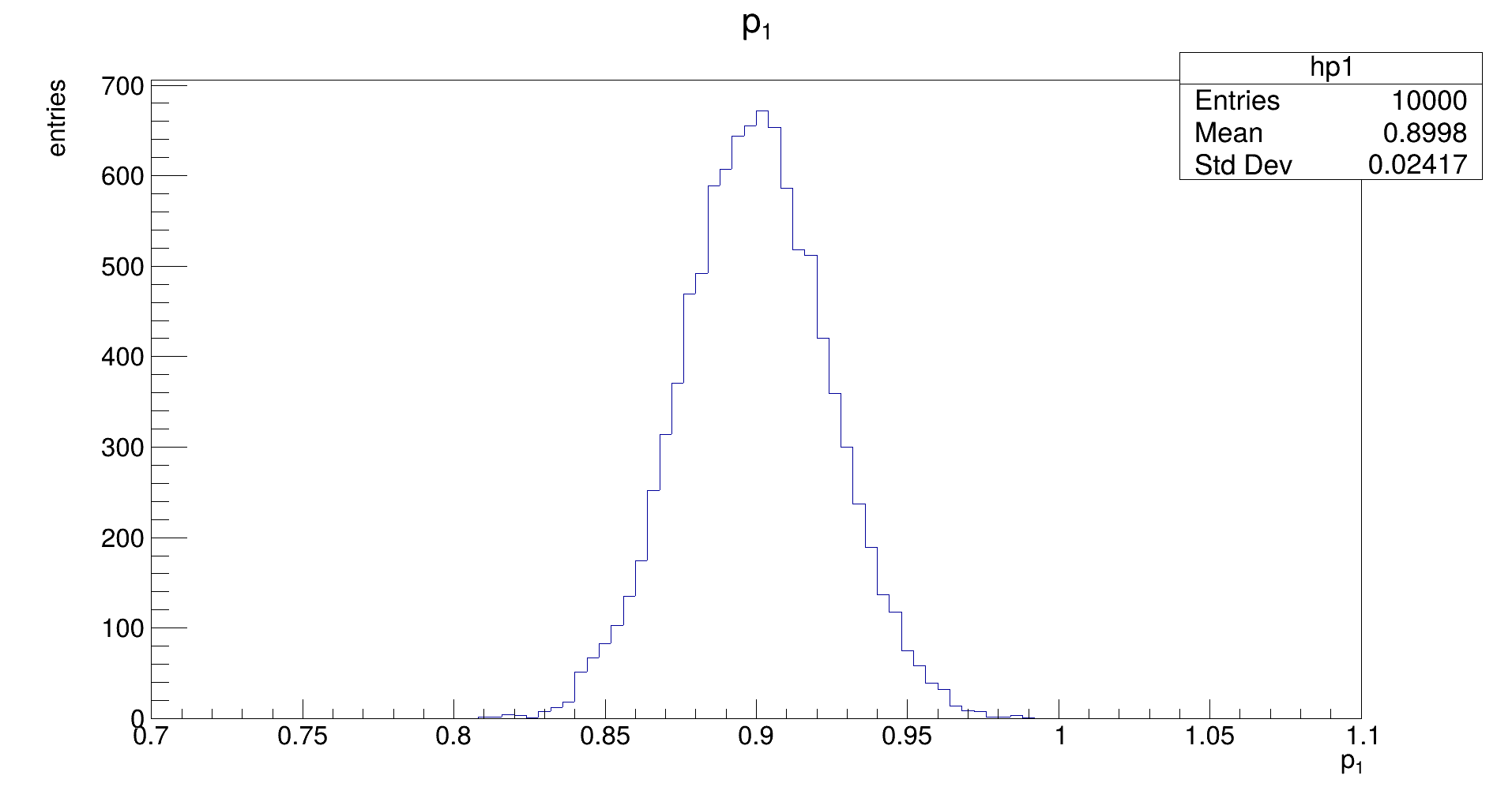
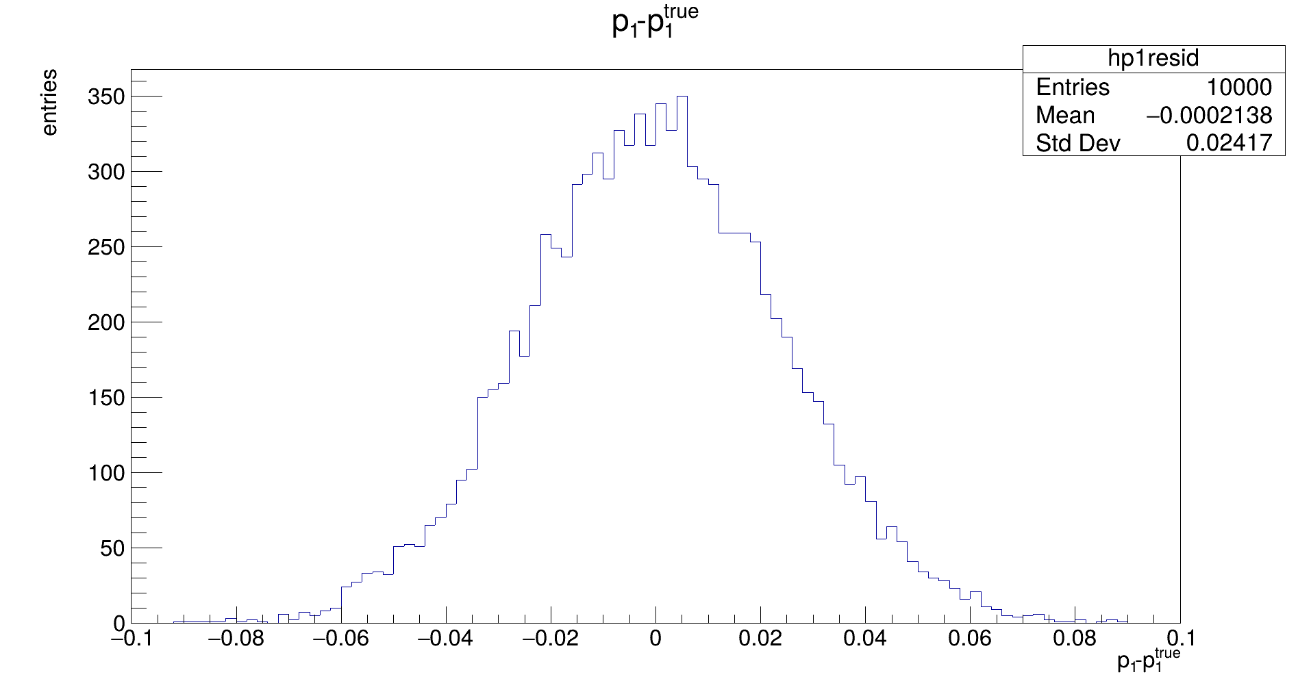
The distribution should be Gaussian, with a mean of the true (generation) value of 𝑝₁, and its width representing the uncertainty that is achievable with the fit. (Note: the latter does not need to be the same as the uncertainty that is estimated by the fit in the covariance.)
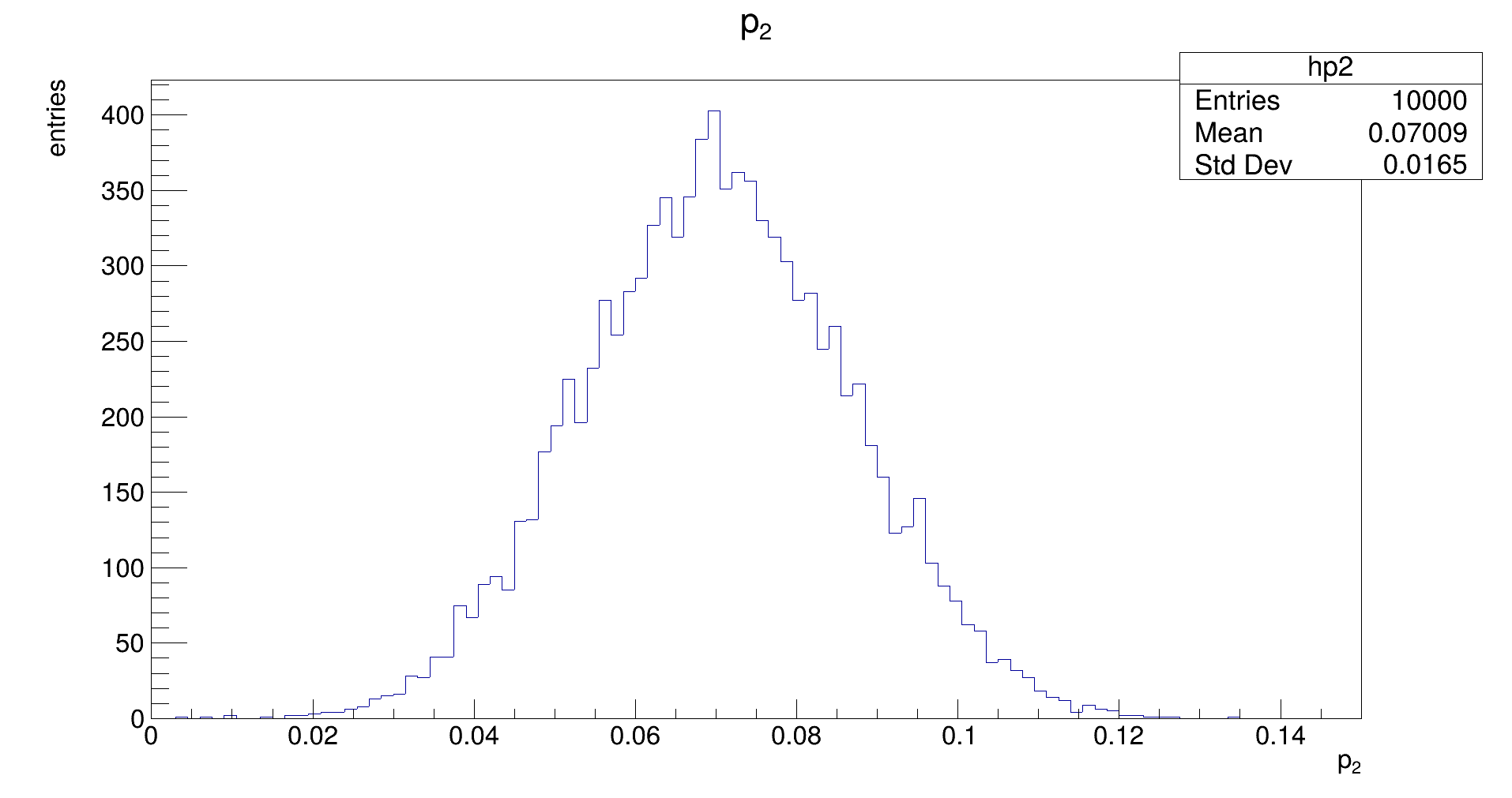
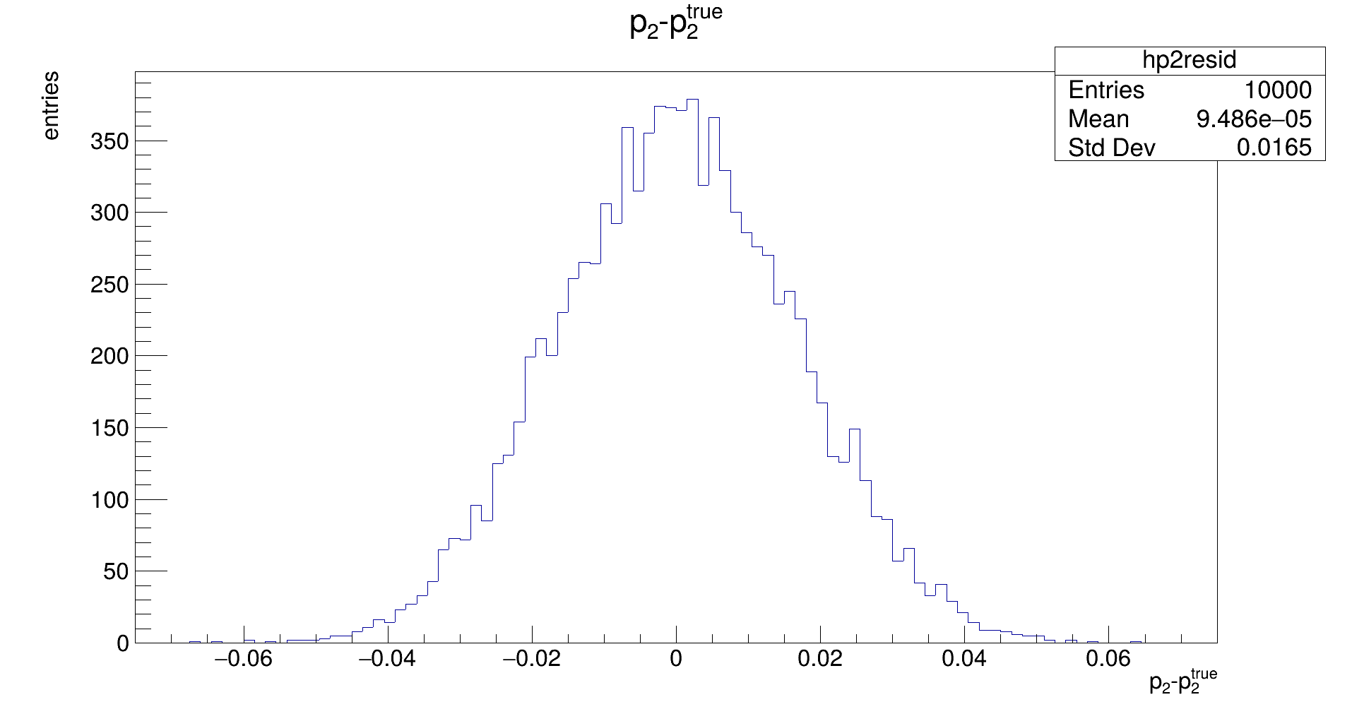
The distribution should be Gaussian, with a mean of the true (generation) value of 𝑝₂, and its width representing the uncertainty that is achievable with the fit. (Note: the latter does not need to be the same as the uncertainty that is estimated by the fit in the covariance.)
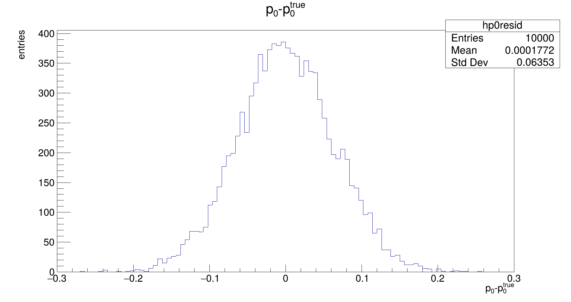
The distribution should be Gaussian, with a mean of 0, and its width representing the uncertainty that is achievable with the fit. (Note: the latter does not need to be the same as the uncertainty that is estimated by the fit in the covariance.) If the mean is not close to zero, the fit returns biased parameters, and will need to be corrected for.
The distribution should be Gaussian, with a mean of 0, and its width representing the uncertainty that is achievable with the fit. (Note: the latter does not need to be the same as the uncertainty that is estimated by the fit in the covariance.) If the mean is not close to zero, the fit returns biased parameters, and will need to be corrected for.
The distribution should be Gaussian, with a mean of 0, and its width representing the uncertainty that is achievable with the fit. (Note: the latter does not need to be the same as the uncertainty that is estimated by the fit in the covariance.) If the mean is not close to zero, the fit returns biased parameters, and will need to be corrected for.
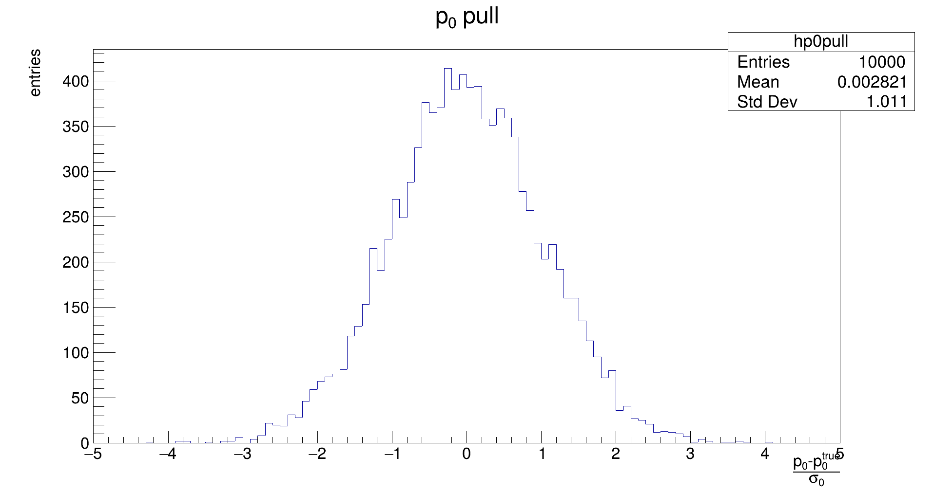
The distribution should be Gaussian, with a mean of 0, and its width should be 1. If the mean is not close to zero, the fit returns biased parameters, and will need to be corrected for. Widths different from 1 indicate if the fit underestimates or overestimates the true error.
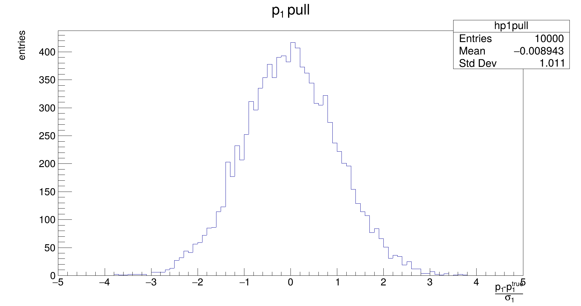
The distribution should be Gaussian, with a mean of 0, and its width should be 1. If the mean is not close to zero, the fit returns biased parameters, and will need to be corrected for. Widths different from 1 indicate if the fit underestimates or overestimates the true error.
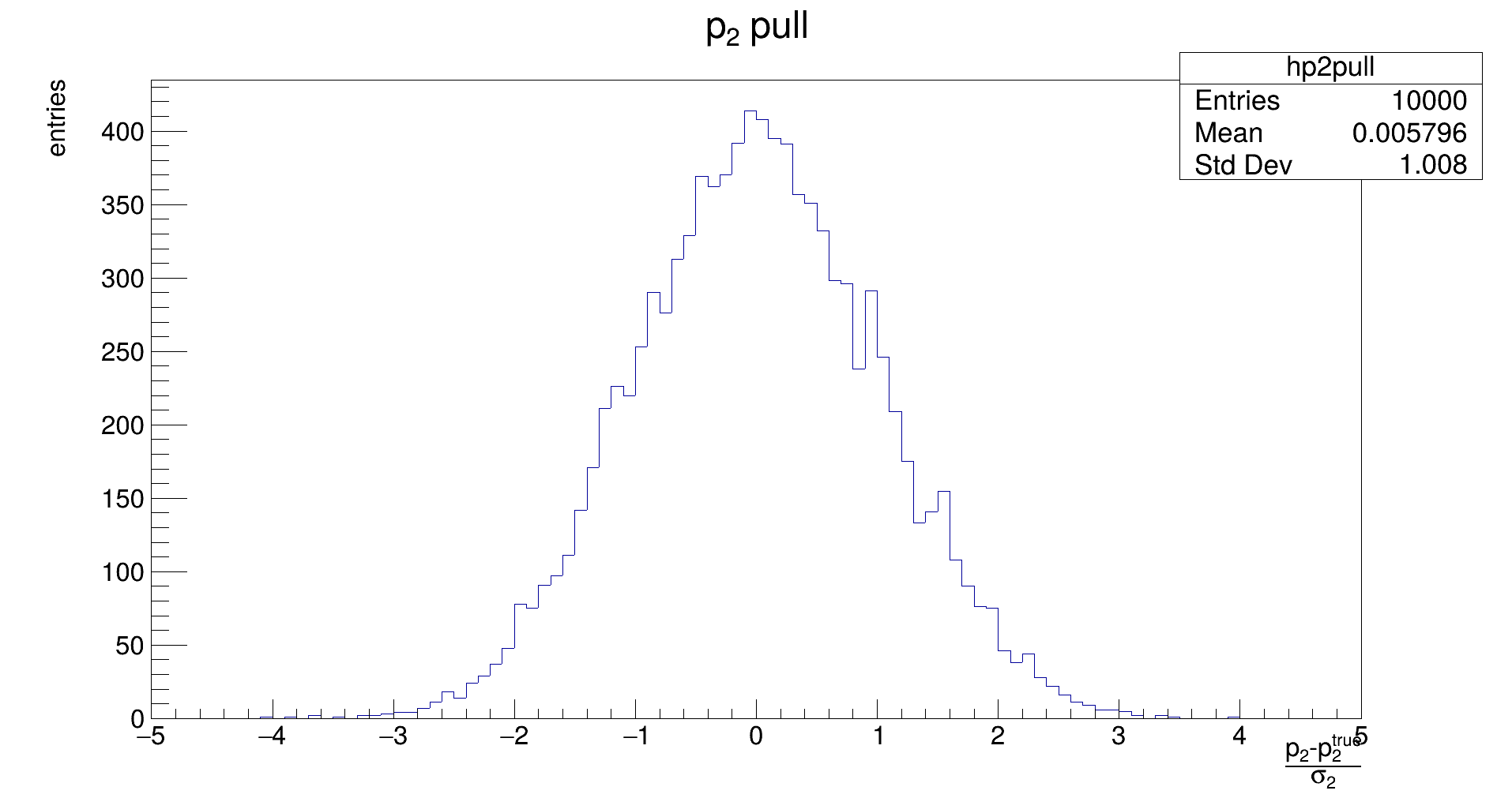
The distribution should be Gaussian, with a mean of 0, and its width should be 1. If the mean is not close to zero, the fit returns biased parameters, and will need to be corrected for. Widths different from 1 indicate if the fit underestimates or overestimates the true error.
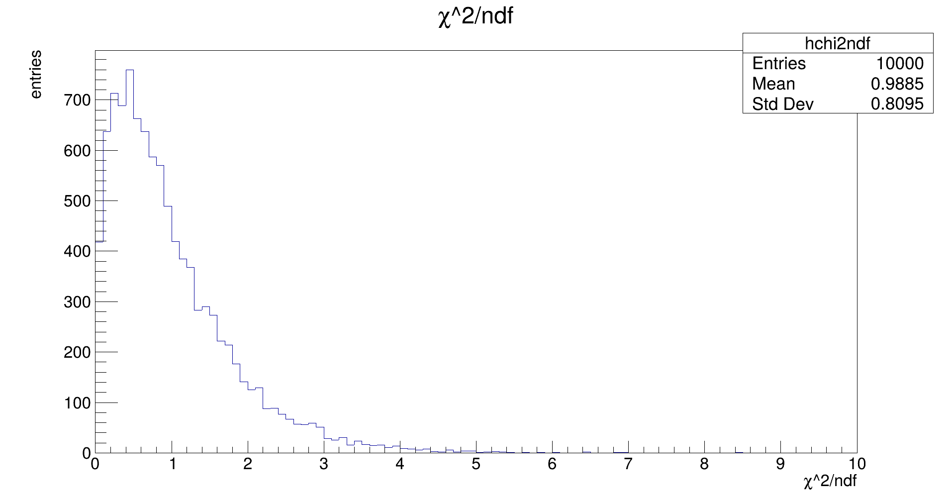
These plots are just scaled versions of each other. One expects the χ² distribution to have a mean of about ndf, or for the χ² / ndf plot, one expects a mean around 1, just as in the plot above.
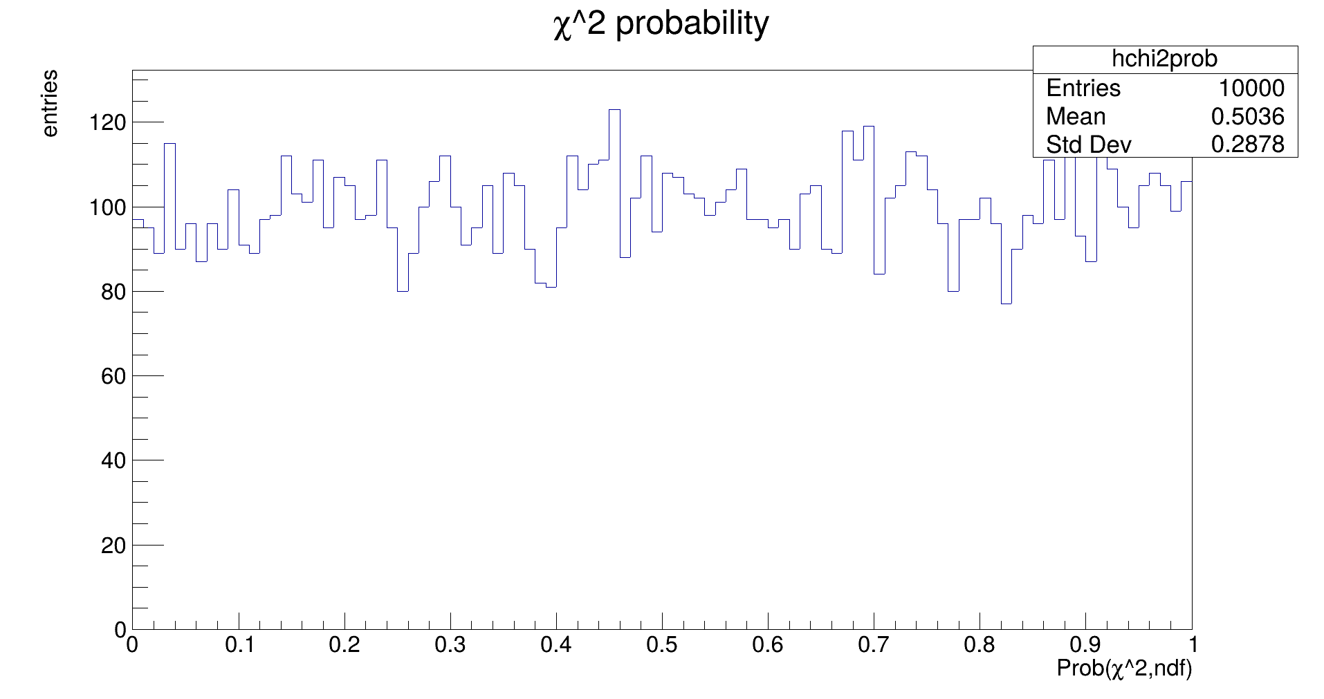
If everything is okay, this plot should be a flat distribution. If the errors of the input measurements are not described correctly, the distribution will develop a distinct migration towards either 1.0 or 0.0. (Try it out by scaling the error used in fitting while keeping the uncertainties in the generation constant!)
We have covered these topics:
To fit correlated measurements, use the χ² derived from multivariate Gaussians (day1) with vector-valued measurements and models.
You should be able to fit any model, as long as the fit parameters enter linearly.
In case the parameters do not enter linearly, if you have a good guess for the parameters from somewhere, you may get away with linearising the model, and fitting and updating parameters iteratively. Or you go with a proper framework like RooFit or MINUIT.
model (𝐩 are fit parameters, fᵢ functions that do not depend on 𝐩):
𝑦(𝑥, 𝐩) = ∑ ᵢ 𝑝ᵢ fᵢ(𝑥)
χ² function
χ² = ∑ ᵢ (𝑥ᵢ − 𝑦(𝑥ᵢ, 𝐩))² / 2σᵢ²
Linear system
/ ⟨ 𝑓₀(𝑥)𝑓₀(𝑥) ⟩ ⟨ 𝑓₀(𝑥)𝑓₁(𝑥) ⟩ ⋯  \ / 𝑝₀ \   / ⟨ 𝑦𝑓₀(𝑥) ⟩ \
| ⟨ 𝑓₀(𝑥)𝑓₁(𝑥) ⟩ ⟨ 𝑓₁(𝑥)𝑓₁(𝑥) ⟩ ⋯  | | 𝑝₁ | = | ⟨ 𝑦𝑓₁(𝑥) ⟩ |
\        ⋮             ⋮        ⋱  / \ ⋮  /   \     ⋮      /